Literature > Basic Principles >

Spectrum Analysis -

Introduction

Canberra offers a variety of nuclear systems which perform data analysis as well as data acquisition. These systems range from small stand alone systems to more sophisticated configurations involving a variety of computer platforms. Typical applications include Environmental Monitoring, Body Burden Analysis, Nuclear Waste Assay, Safeguards and other applications. The following section presents some of the typical procedures and calculations involved in nuclear applications.

Counting Statistics

Radioactive decay occurs randomly in time, so the measurement of the number of events detected in a given time period is never exact, but represents an average value with some uncertainty. Better average values can be obtained by acquiring data over longer time periods. But, since this is not always possible, it is necessary to be able to estimate the accuracy of any given average.

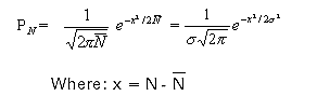
Nuclear events follow a Poisson distribution which is the limiting case of a binomial distribution for an infinite number of time intervals, and closely resembles a Gaussian distribution when the number of observed events is large. The Poisson distribution for observing N events when the average is N, is given by:

and has standard deviation s (sigma) equal to . A graph of P_N for equal to 3 and to 10 is shown in Figure 1.50. The curves are asymmetric and have the property that is not exactly the most probable value but is close to it. However, as N increases the curve becomes more symmetric, and approaches the Gaussian distribution:

The integral of the area under the Gaussian curve is often used to report errors in terms of a confidence level in percent. For example, in the value reported as 64 ± 8, 8 is equal to s and represents 68% of the area under the appropriate Gaussian curve for N=64. It may be stated as the value one is 68% confident of obtaining if the measurement is repeated. Traditionally, many of Canberra’s MCAs have used 1.65 s, which corresponds to a 90% confidence level. Probable error is often used, which corresponds to a 50% confidence level. These can be user-set to other values, such as:

Value of s	% Confidence
0.68	50.0
1.00	68.3
1.15	75.0
1.65	90.0
1.96	95.0

Since the uncertainty depends upon the square root of the counts, improvements in accuracy by counting longer, or by using a more efficient detector, only increase as the square root. For example, if 564 counts are obtained in an hour for s = » 24 for a 24/564 = 4.3% accuracy, counting for two hours to get 1133 counts with s » 34 only gives an improvement to 3.0%. In other words, counting twice as long gives an improvement of 1/ = 0.71, or 29%.

Examples of data in which counting statistics apply include: the counts in a counter, the counts in a single channel of an MCA spectrum, or the sum of counts in a group of channels in an MCA spectrum. The situation becomes even more complicated when subtracting a background as shown in the following separate, but frequent, cases.

• Subtracting background counts, as in one counter’s value from another, or for each channel (when subtracting one spectrum from another).
• Subtracting a straight line background from a peak on top of the background in a spectrum, such as a HPGe peak on top of Compton pulses from higher energy gamma rays.

The error in adding or subtracting two numbers with errors, as in:

is given by:

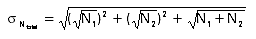
Consider a low level counting situation in which 56 counts are obtained in 10 minutes, and a background of 38 counts in 10 minutes was measured without the sample. The result is 56-38 = 18 counts, with an error of ⁼ or approximately 9.7, a s value of 54%.

A better procedure is to measure the background over a longer period of time to obtain a small percentage error and factor to the appropriate time for each sample analyzed. Using the same example as above, but with a 100 minute background of 380 counts, the result would be 56-(380/10) = 18 counts, with an error of

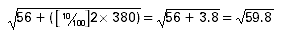
or approximately 7.7, a s value of 43%.

Net Area Calculation

For the case in which a peak lies on a background that cannot be subtracted by a background spectrum, such as shown in Figure 1.51 for an MCA spectrum from a HPGe detector:

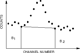
Figure 1.51
Net Area Determination

The area above the background represents the total counts between the vertical lines minus the trapezoidal area below the straight line. If the total counts are P and the end-points of the straight line are B₁ and B₂, then the net area is given by:

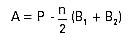
Where n = The number of channels between B₁ and B₂.

It is tempting to calculate the uncertainty by just using the formula for subtracting two numbers, with standard deviations of:

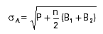
However, this is incorrect because the error in the trapezoidal area is not just square root of the counts, but depends upon how the errors in B₁ and B₂ affect the straight line across the entire region. The proper procedure, which is implemented in Canberra MCAs and in analysis of peak areas in various HPGe software packages, is derived as follows:

The standard deviation in a function A is given by:

A = f(N₁ N₂ ...Nn)

where N_n is the counts in channel N.

The estimate of the standard deviation in A is given by:

Where P₁...P_n are the channels in the peak (inside B₁ and B₂).

End-Point Averaging

If the background is large compared to the peak area, a better determination of background can be made by averaging over several channels. If B₁ is the sum of counts over n₁ channels, and B₂ over n₂ channels, the area is then:

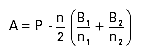
and the standard deviation is:

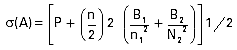
Most Canberra MCAs and analysis software packages perform end-point averaging with a user-selectable number of end-points.

There are many ways of calculating the net counts under a peak. The method described above is a valid, common method, provided that there are no interferences from photopeaks adjacent to the peak of interest, and assuming that the background continuum varies linearly from one side of the peak to the other.

However, if interferences exist, other methods of calculating the net area of a peak must be employed which can include, (but are not limited to), the use of parabolic or step background algorithms, as well as non-linear fitting algorithms, etc. For further discussions concerning these techniques and others, the reader is referred to more detailed texts and formal spectroscopy training courses.

Energy Calibration

Many nuclear applications require a means for determining the energy at a particular channel location of a spectrum. To meet this need, Canberra has implemented various techniques which are briefly discussed below.

In some MCAs, a simple two-point energy calibration is used to determine both the offset and slope by the equation:

E = A(ch) + B

Where: ch = channel number

Thus, the energy vs. channel number can be directly read out. However, the more advanced MCA Systems, like the Genie 2000 and Genie-ESP Network allow users to choose between first-order (i.e. linear) or second-order (i.e. quadratic) equations that use a least squares fit to multiple data points.

Most preamplifier, amplifier and ADC systems are very linear and first-order energy calibration can properly describe the data. For example, a Canberra germanium detector with 2002 Preamplifier, 2025 Amplifier and 8701 ADC has nonlinearities less than 0.05% for the preamplifier and amplifier, and 0.025% for the ADC. The combined nonlinearity is then:

This is still a very small number, but for a spectrum of 4000 channels, the low and high energy channels may be correct and leave a 0.00075 x 2000 = 1.5 channel uncertainty at channel 2000. A second-order term in the energy calibration can remove this in order to provide very accurate energy-channel calibration over the entire range, according to the equation:

E = A(ch)² + B(ch) + C

Where: ch = channel number

A further refinement is provided by using least-squares techniques to determine the equation that best fits the data, when more than the minimum number of points is available, (2 for first-order, 3 for second-order). The AccuSpec, Genie 2000 and Genie-ESP MCA Systems use this technique.

Nuclide Identification and Quantitative Analysis

Many applications with high purity germanium (HPGe) detector spectra involve identifying particular gamma rays with specific nuclides. The sharp peaks in the HPGe spectra, coupled with a careful precise energy calibration, can be used for generally unique determinations of the nuclides in a sample. If an automatic peak search capability is provided then a complete sample analysis can be accomplished without operator intervention, which is ideal for analyzing large numbers of samples. All Canberra HPGe/computer-based gamma spectroscopy systems provide nuclide identification through peak searches of spectra and scans of standard and user-generated nuclide libraries. A sample printout of a Genie 2000 nuclide identification report is shown in Figure 1.52.

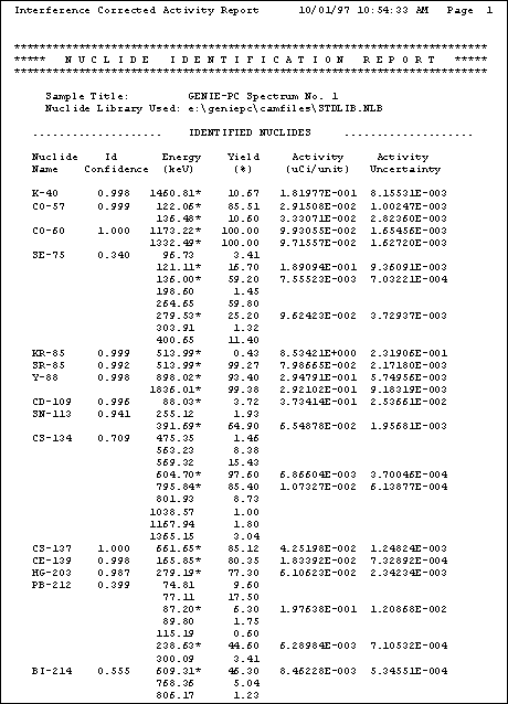
Figure 1.52
Isotope ID

In the Genie 2000 and VMS-based platforms, the peak search locates peak centroids and then enters a region of interest about each peak. This is especially useful for observing the quality of data obtained. Canberra analysis software provides the additional capability of resolving overlapping peaks into individual components.

The final step in nuclide analysis is to determine the intensity of the radioactivity corresponding to each isotope. The net area of the peak is directly related to the intensity, but it is also necessary to correct for the efficiency of the detector, the branching ratio of the source, and the half life (if it is desired to relate the activity to an earlier or later time). The efficiency was discussed earlier and has an energy dependence such as shown in Figure 1.1. The branching ratio (or yield) is used to correct the number of gamma rays observed to obtain the number of disintegrations of the source. Figure 1.53 shows the decay scheme for ⁸⁸Y and the percent of disintegrations leading to the various gamma rays.

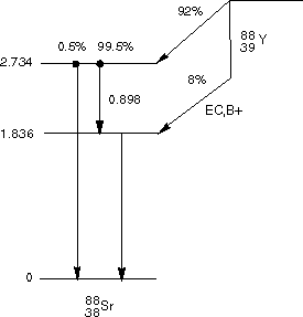
Figure 1.53
⁸⁸Y Decay Scheme

The activity of a particular isotope is given in microcuries as:

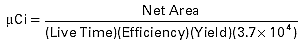
Where yield is the branching ratio fraction and live time is the actual ADC live time disintegrations per second. Half-life corrections are made by multiplying an exponential factor.

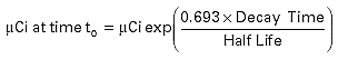
Where decay time and half-life must be in the same units (seconds, minutes, hours, or years).

Further specific data analysis is highly dependent upon the application, detector and electronics configuration, and is beyond the scope of this brief presentation.

Efficiency Calibration

In the equation for activity cited above, the value for efficiency is dependent on the geometry of the sample - size, density, and distance from detector. For the detectors used in gamma analysis, efficiency varies significantly with energy (see Figure 1.1).

Therefore, each counting geometry requires an efficiency calibration, using a known standard in the same geometry which includes multiple energies. A series of data pairs of efficiency vs. energy are generated from the relationship:

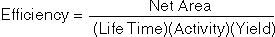
Where Activity is the strength (in Bq) of the standard source (at collection time) at the given energy, yield is the branching ratio fraction and live time is the actual ADC live time.

In the Genie software system, the calibration data from the standard are entered into a "Certificate File", with these data being used for subsequent efficiency calibrations. The software will automatically correct for source decay by the formula:

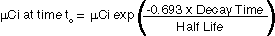
Where decay time and half-life are in the same units (seconds, minutes, hours, or years).

From the series of data pairs, a curve of efficiency versus energy is generated, with the user having a choice of fitting paradigms. Thus, the software can calculate efficiency at any energy in the calibrated energy range when analyzing an unknown spectrum.

Minimal Detectable Activity

The calculation of Minimum Detectable Activity for a given nuclide, at the 95% confidence level, is usually based on Currie’s derivation (Currie, L.A. (1968) Anal. Chem. 40:586.), with one simplified formulation being:

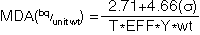
where:

• s is the standard deviation of the background at the energy of interest
• T is the collect time (sec)
• EFF is the efficiency at the energy of interest
• Y is the Branching Ratio wt is sample weight

This formulation takes into account both kinds of errors - false positive and false negative, and yields the smallest level of activity which can be detected with 95% confidence, while also having 95% confidence that "activity" is not detected falsely from a null sample. When the measurement is made on a ‘blank’, with no activity, but with the same form and density as an actual sample, the calculated MDA is an a priori estimate of the best sensitivity that can be expected from sample measurements. When the calculation is applied to a spectrum collected from an actual sample, the background at the energy of interest will in most cases be higher, due to interference and Compton scattering from other nuclides in the sample. Thus, the MDA for an actual sample, computed a posteriori, will be somewhat higher than the a priori estimate.

The MDA - also referred to as Lower Limit of Detection (LLD) - can be improved by increasing the efficiency of detection, decreasing the background, or, for a given experimental setup, by increasing the collect time. It is frequently necessary to select the appropriate collect time to ensure that the measured MDA will be below the action level mandated by the count-room procedures.

The above formula for MDA, generally accepted in the United States and many other countries, is implemented in a more complete form in Canberra Analytical software. Some Canberra software packages, such as Genie 2000, offer the user a choice of additional formulas required in other countries.