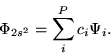
| (1) |
Darío M. Mitnik
Departmento de Física, FCEyN, Universidad de Buenos Aires,
(C1428EGA) Buenos Aires, Argentina
and
Instituto de Astronomía y Física del Espacio (IAFE),
Casilla de Correo 67, Sucursal 28,
(C1428EGA) Buenos Aires, Argentina.
32.80.Dz, 31.70.Hq
Published in Physical Review A 70, 022703 (2004)
Among the fully quantum nonperturbative theories, the time-dependent close-coupling (TDCC) method has been successfully employed for calculations of electron-impact ionization [1,2,3]. We have recently [4] studied the dielectronic capture into doubly excited resonances within the time-dependent framework. This study required the development of methods for generating accurate wave functions for doubly excited autoionizing states and time-dependent close-coupling calculations of the capture and the subsequent decay of autoionizing states. Since in future applications we wish to consider resonances in the time-dependent framework and to study processes that involve transitions to and among continuum states, we chose to discretize the wave functions and the action of operators which result from these procedures, working therefore in a numerical lattice, thus solving the problem of an ion inside a box.
Solving real atomic-physical problems with discrete numerical methods is an approximation that relies on strong logical grounds. It becomes a very good approximation to the physical bound states for all orbitals that fit well into the lattice (i.e., for such bound states in which the wave function at the boundaries approaches zero in a practical sense for numerical calculations). Use of discrete lattice functions allows the system to be described by the dynamics of always-square-integrable functions. Even if the states can be represented by fully analytical functions (such as the hypergeometrical functions for the continuum Coulomb waves), a proper calculation with these functions could involve a numerical work, and therefore, finite-lattice discretization. The method presented here has many other important advantages. It gives the exact solutions to the problem of an ion confined in a box. If the discretized allowed energy levels are positive, the eigenfunctions are true continuum solutions of the ion, not necessarily confined inside a box. These solutions form a set selected by a particular boundary condition, i.e., these are the particular true continuum wave functions with zero value at the boundaries of the box. All the solutions obtained by direct diagonalization are naturally orthogonal, and most importantly, the set is complete. Finally, the simplicity of the method is expected to lead to a greater understanding of the close-coupling formalism in general.
The problem of a spatially confined system has been a subject of interest in many branches of physics and chemistry since the early years of quantum mechanics. Nowadays, investigations on confined systems in physics (see, for example, [5]) have focused especially on the study of artificial atoms, also known as quantum dots (essentially a number of electrons confined in a potential well). However, an important theoretical motivation for the study of enclosed systems is to understand in detail the electron correlation effects on the properties of those systems.
In this work, we study how to obtain the exact wave functions in two-electron systems by the direct solution of the Schrödinger equation. Two methods are developed for this purpose. The first method consists of the direct diagonalization of the two-electron Hamiltonian on the radial grid. The second method is a constrained relaxation of the wave functions, until they relax on the successive doubly excited levels of He. The relaxation method was currently used in the TDCC method for calculation of the ground and first excited states of ions, and also for calculation of ground and low-lying excited states in Bose-Einstein condensates [6]. However, a particular treatment is needed for calculation of doubly excited levels.
In order to explain the main features of the different methods, a detailed presentation of the theory is given for the spherically symmetric model [7,8] (also known as the Temkin-Poet model or the S-wave model). The remainder of the paper is the following. Section [3] shows the results for the first doubly excited wave functions obtained in both methods. Section [3b] shows how to use the Feshbach projection-operator formalism in order to compare the results obtained in both methods. In Sec. [3c] we propagate the first doubly excited autoionizing level, showing how the autoionization process evolves in time, and we also calculate the autoionization rate from this level by monitoring the autocorrelation function in time.
We first solve this problem by a direct diagonalization
of the Hamiltonian,
 |
(3) |
| (5) |
| (6) |
where the diagonal elements
![]() are:
are:
| (9) |
| (10) |
The complete set of wave functions corresponding to the
S-wave model He are obtained from the direct diagonalization of the
matrix ![]() [Eq. (8)].
Standard diagonalization subroutines [9]
produce a matrix
[Eq. (8)].
Standard diagonalization subroutines [9]
produce a matrix ![]() with rank
with rank
![]() where the column
where the column
![]() is the
is the ![]() eigenvector of the Hamiltonian.
In this case, the value of the
eigenvector
eigenvector of the Hamiltonian.
In this case, the value of the
eigenvector ![]() at the
at the ![]() point in the numerical grid is
given by
point in the numerical grid is
given by
| (11) |
In order to allow the diagonalization of large matrices, we wrote the
computer programs to use on distributed-memory parallel computers.
The Hamiltonian matrix is directly partitioned over the many processors,
so memory requirements per processor are minimized and scalability in
time is achieved. The procedure used in the parallelization of the
codes is similar to that employed for the parallelization of the
![]() -matrix package [10].
-matrix package [10].
 |
(14) |
Since
![]() , the net result from this imaginary time
propagation is the enhancement of those components of the solution with smaller
eigenvalues of
, the net result from this imaginary time
propagation is the enhancement of those components of the solution with smaller
eigenvalues of ![]() relative to those with larger eigenvalues.
At the limit
relative to those with larger eigenvalues.
At the limit
![]() ,
,
![]() .
Thus, after many iterations (renormalizing continuously the wave function),
only the lowest level eigenvalue (i.e., the ground state, or the first
metastable level, according to the parity of the initial function
.
Thus, after many iterations (renormalizing continuously the wave function),
only the lowest level eigenvalue (i.e., the ground state, or the first
metastable level, according to the parity of the initial function ![]() )
survives from the relaxation.
Higher eigenvectors can be calculated by imposing
constraints at the iteration of the relaxation which requires
the state to be orthogonal, thus preventing its collapse to lower levels.
This procedure is a well-known method which has been employed to determine
energies of atomic and molecular systems [12],
as well as the ground-state energy of a quartic oscillator [13].
In particular, for the case of He, Kulander et al. [14]
integrated Hartree-Fock time-dependent equations in imaginary time, to
obtain the
)
survives from the relaxation.
Higher eigenvectors can be calculated by imposing
constraints at the iteration of the relaxation which requires
the state to be orthogonal, thus preventing its collapse to lower levels.
This procedure is a well-known method which has been employed to determine
energies of atomic and molecular systems [12],
as well as the ground-state energy of a quartic oscillator [13].
In particular, for the case of He, Kulander et al. [14]
integrated Hartree-Fock time-dependent equations in imaginary time, to
obtain the ![]() S ground state,
and Bottcher et al. [15] calculated the energies
of the
S ground state,
and Bottcher et al. [15] calculated the energies
of the ![]() S, and the
S, and the ![]() S
and
S
and ![]() P singly excited levels,
by relaxing coupled Hylleras-type functions with a damping kinetic operator.
P singly excited levels,
by relaxing coupled Hylleras-type functions with a damping kinetic operator.
The relaxation method, however, will work well for the low-lying
single-excited levels (e.g., ![]() ), but not for the doubly excited levels.
The reason for that is that the orthogonalization procedure becomes unstable,
even for a relatively low number of wave functions.
In general, the relaxed wave function will collapse in any of the
), but not for the doubly excited levels.
The reason for that is that the orthogonalization procedure becomes unstable,
even for a relatively low number of wave functions.
In general, the relaxed wave function will collapse in any of the ![]() bound
levels, or any of the
bound
levels, or any of the ![]() continuum levels, without any warranty that
this procedure will ends in a doubly excited level.
doubly excited autoionizing states are calculated by imposing
additional constraints at the iteration of the relaxation, projecting out
also the one-electron component of the lower wave functions.
Therefore, we do not allow the function to have any
continuum levels, without any warranty that
this procedure will ends in a doubly excited level.
doubly excited autoionizing states are calculated by imposing
additional constraints at the iteration of the relaxation, projecting out
also the one-electron component of the lower wave functions.
Therefore, we do not allow the function to have any ![]() component
in any of the radial coordenates.
The relaxation of coupled Hylleras-type functions with a damping kinetic
operator procedure was used by Schultz et al. [16]
for the calculation of the
component
in any of the radial coordenates.
The relaxation of coupled Hylleras-type functions with a damping kinetic
operator procedure was used by Schultz et al. [16]
for the calculation of the ![]() autoionizing level of He.
In this paper, the authors outlined the basic theoretical method
without providing broad details concerning the computationally procedures.
However, we found that this technique requires particular care in order to
obtain convergent results and deserves detailed explanations of the
computational algorithm employed.
Based on our experience, the suggested receipt for calculating (for example)
the
autoionizing level of He.
In this paper, the authors outlined the basic theoretical method
without providing broad details concerning the computationally procedures.
However, we found that this technique requires particular care in order to
obtain convergent results and deserves detailed explanations of the
computational algorithm employed.
Based on our experience, the suggested receipt for calculating (for example)
the ![]() wave function (corresponding to the
wave function (corresponding to the ![]() level) is the
following
level) is the
following
| (15) |
| (17) |
 |
(21) |
The computer codes which implement this method are also adapted to run on parallel computers. In this case, the wave functions are partitioned over the many processors in such a way that the communications between the processors are minimized and performed at every time step only for the partitioned domain borders. This parallelization scheme is a standard procedure for many of the TDCC different works (see, for example [18]).
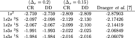
We have computed first the ground state of the S-wave model He with
different numerical grids in order to check the sensitivity and
convergence of the calculations and the compatibility of the
two different numerical methods.
Table I shows that the energy of the ![]() level,
obtained with a numerical grid having a mesh spacing
level,
obtained with a numerical grid having a mesh spacing
![]() is
is
![]() a.u., compared with the
best value available in the literature of
a.u., compared with the
best value available in the literature of
![]() a.u. (with 14 other digits that are not relevant in our
comparisons) obtained by Goldman [19].
It is important to notice that for this numerical lattice, the one-electron
energy of the He
a.u. (with 14 other digits that are not relevant in our
comparisons) obtained by Goldman [19].
It is important to notice that for this numerical lattice, the one-electron
energy of the He![]()
![]() level is
level is
![]() a.u., compared to
the exact value of
a.u., compared to
the exact value of ![]() au.
We found an excellent agreement between the results obtained with the
constrained relaxation method and with the direct diagonalization method.
We performed a better calculation, with a mesh size of
au.
We found an excellent agreement between the results obtained with the
constrained relaxation method and with the direct diagonalization method.
We performed a better calculation, with a mesh size of
![]() a.u., where
a.u., where
![]() a.u.,
and obtained a ground-state energy of
a.u.,
and obtained a ground-state energy of
![]() a.u. with both theoretical methods.
Better energies can be generated by decreasing the mesh step size and
increasing the number of points.
Convergence is demonstrated by using a grid with
a.u. with both theoretical methods.
Better energies can be generated by decreasing the mesh step size and
increasing the number of points.
Convergence is demonstrated by using a grid with
![]() a.u., where
a.u., where
![]() a.u.
and
a.u.
and
![]() a.u.,
and with
a.u.,
and with
![]() , in which
, in which
![]() a.u.
and
a.u.
and
![]() a.u.
Table I also shows the energies for the first excited
levels
a.u.
Table I also shows the energies for the first excited
levels ![]() and
and ![]() , for both the singlet and triplet terms.
The results are in good agreement with the results given by Draeger,
up to a 2% error.
, for both the singlet and triplet terms.
The results are in good agreement with the results given by Draeger,
up to a 2% error.
|
Figure 1
shows the probability densities of the first
wave functions obtained with the direct diagonalization method,
for the numerical grid with a mesh spacing
![]() a.u., and a number of
a.u., and a number of ![]() points.
We show only one set of figures because the wave functions obtained from
both methods, for these levels, are indistinguishable.
We used the same numerical grid to calculate the energies of the He
points.
We show only one set of figures because the wave functions obtained from
both methods, for these levels, are indistinguishable.
We used the same numerical grid to calculate the energies of the He![]()
![]() level and found five bound orbitals (
level and found five bound orbitals (![]() to
to ![]() ), therefore we
expect the plots of the figures to be similar to those obtained without
a confining box.
), therefore we
expect the plots of the figures to be similar to those obtained without
a confining box.
We have computed the energy of many doubly excited states
by direct diagonalization, and after the proper identification of the states,
we compared them with the results obtained with the relaxation method.
The numerical grid having a mesh spacing
![]() and a number of
and a number of ![]() points has 57 negative eigenenergies.
Many of their eigenfunctions are bound functions of the form
points has 57 negative eigenenergies.
Many of their eigenfunctions are bound functions of the form ![]() ,
and most of them are single-continuum wave functions of the form
,
and most of them are single-continuum wave functions of the form ![]() .
We also found in this group of functions with negative energy
doubly excited levels corresponding to
.
We also found in this group of functions with negative energy
doubly excited levels corresponding to ![]() ,
, ![]() , and
, and ![]() .
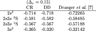
Table II shows the results of the calculated energies
for the first doubly excited levels in the S-wave model He. Very good agreement is obtained for the
.
Table II shows the results of the calculated energies
for the first doubly excited levels in the S-wave model He. Very good agreement is obtained for the ![]() terms
(both singlet and triplet) between the constrained relaxation and the
direct diagonalization results.
terms
(both singlet and triplet) between the constrained relaxation and the
direct diagonalization results.
|
The probability density of these wave functions, obtained with the
relaxation method, is shown in Figure
2.
Among the 57 negative-energy levels obtained with the diagonalization,
we can easily identify the ![]() and
and ![]() functions.
It is also very simple to find the
functions.
It is also very simple to find the ![]() wave function by direct inspection
between the many continuum functions.
This is shown in
Fig. 3,
where the
wave function by direct inspection
between the many continuum functions.
This is shown in
Fig. 3,
where the ![]() through
through ![]() wave functions (with eigenvalues
wave functions (with eigenvalues
![]() ,
, ![]() ,
, ![]() , and
, and ![]() a.u., respectively)
are plotted.
However, for the
a.u., respectively)
are plotted.
However, for the ![]() level, the functions calculated with both theoretical
methods are different.
In the next section, we will establish the relationship between them.
level, the functions calculated with both theoretical
methods are different.
In the next section, we will establish the relationship between them.
Figure 4 shows, in a detailed scale,
the first doubly excited wave function
![]() obtained with the constrained damped
relaxation method (a), and
obtained with the constrained damped
relaxation method (a), and ![]() , obtained with the direct
diagonalization method (b).
It is noticeable that both functions are different because the
relaxed function
, obtained with the direct
diagonalization method (b).
It is noticeable that both functions are different because the
relaxed function ![]() is a ``pure" bound function
which does not contain any interaction with the continuum.
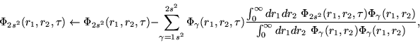
Following Fano [21], we will observe that both functions
are related by
is a ``pure" bound function
which does not contain any interaction with the continuum.
Following Fano [21], we will observe that both functions
are related by
In order to test the results obtained for the ![]() wave functions
with both methods, we employ a Feshbach projection formalism,
but in a way inverse to the procedure used by Fano [21].
In general, the problem is how to obtain the true eigenvector
wave functions
with both methods, we employ a Feshbach projection formalism,
but in a way inverse to the procedure used by Fano [21].
In general, the problem is how to obtain the true eigenvector ![]() of the total Hamiltonian, starting from the restricted
functions
of the total Hamiltonian, starting from the restricted
functions ![]() , and combining them as expressed in Eq.
(22).
Here, we will obtain the restricted
, and combining them as expressed in Eq.
(22).
Here, we will obtain the restricted ![]() wave function from the
eigenfunction of the total Hamiltonian (the wave function
wave function from the
eigenfunction of the total Hamiltonian (the wave function ![]() ).
That is equivalent to projecting the eigenfunction
).
That is equivalent to projecting the eigenfunction ![]() onto
the subspace
onto
the subspace ![]() , where
, where ![]() . The procedure applied in order
to obtain the projected wave
. The procedure applied in order
to obtain the projected wave
![]() is to calculate
is to calculate
| (23) | |||
If the numerical procedures are correct, the new wave function
![]() must be very similar to the
must be very similar to the
![]() wave function obtained from the relaxation method.
Graphic results of the probability densities for the functions
wave function obtained from the relaxation method.
Graphic results of the probability densities for the functions
![]() and
and
![]() are shown in
Fig. 5.
It is clear that the
are shown in
Fig. 5.
It is clear that the
![]() function is very similar to the
function is very similar to the
![]() function displayed in Fig.
2
(first figure).
On the other hand, the
function displayed in Fig.
2
(first figure).
On the other hand, the
![]() function has the form of
a
function has the form of
a ![]() function, like the second of the continuum functions displayed in
Figure 3.
The overlap between the
function, like the second of the continuum functions displayed in
Figure 3.
The overlap between the ![]() function (obtained by diagonalization)
and the
function (obtained by diagonalization)
and the ![]() function (obtained by relaxation)
is
function (obtained by relaxation)
is
![]() , which
accounts for all the
, which
accounts for all the ![]() components presented in the eigenvector
components presented in the eigenvector
![]() .
The overlap of the relaxed function with the new projected function is
.
The overlap of the relaxed function with the new projected function is
![]() , an indication
of the great similarity between the relaxed and the Feshbach projected
functions.
It is also consistent with the fact that
the overlap
, an indication
of the great similarity between the relaxed and the Feshbach projected
functions.
It is also consistent with the fact that
the overlap
![]() ,
meaning that the projection mechanism in the relaxation did not eliminate
completely the
,
meaning that the projection mechanism in the relaxation did not eliminate
completely the ![]() components.
components.
As we propagate the Schrödinger equation in imaginary time
[Eq.(13)], we approach the (real) energy of the
doubly excited level.
We need to propagate it further in real time in order to
obtain the imaginary part of the energies, i.e., the lifetime
of the level.
Figure 6 shows the evolution of the
probability density of the wave function
![]() under the time propagation with the Schrödinger equation,
under the time propagation with the Schrödinger equation,
The different frames of the figure show snapshots at early times from the
beginning of the propagation.
The velocity of the autoionizing electron can be obtained approximately
from the energy difference between the ![]() level and the He
level and the He![]() ground state, i.e.,
ground state, i.e.,
![]() , where
, where
![]() a.u.
is the energy of the free electron. That gives a velocity of 1.6 a.u. for
the free autoionized electron.
Taking into account the size of the box (22.5 a.u.),
this free electron will rebound from the box borders at an approximate time
of 14 a.u.
Snapshots of the propagation of the
a.u.
is the energy of the free electron. That gives a velocity of 1.6 a.u. for
the free autoionized electron.
Taking into account the size of the box (22.5 a.u.),
this free electron will rebound from the box borders at an approximate time
of 14 a.u.
Snapshots of the propagation of the
![]() wave function are
shown at the times 3.6, 7.3, 10.8, and 14.4 a.u..
The pictures show how the initial pure
wave function are
shown at the times 3.6, 7.3, 10.8, and 14.4 a.u..
The pictures show how the initial pure ![]() wave function acquires a
continuum feature, as it evolved in time. At the beginning, a
slow deformation of the wave is developed, with the probability dropping
through the wings of the wave. Then, the characteristic pattern of a
wave function acquires a
continuum feature, as it evolved in time. At the beginning, a
slow deformation of the wave is developed, with the probability dropping
through the wings of the wave. Then, the characteristic pattern of a
![]() continuum wave is formed at the axes, advancing rapidly to
the box borders.
After this time, the wave function bounces back and we found oscillations
which under specific conditions can return the propagated function to
roughly the original shape at particular times.
We are aware of the possibility of introducing a mask function in order to
absorb the wave at the borders preventing the rebound, but this revival
of the original wave function can have a particular further interest.
The full movie for the propagation can be downloaded at
the author's personal webpage:
continuum wave is formed at the axes, advancing rapidly to
the box borders.
After this time, the wave function bounces back and we found oscillations
which under specific conditions can return the propagated function to
roughly the original shape at particular times.
We are aware of the possibility of introducing a mask function in order to
absorb the wave at the borders preventing the rebound, but this revival
of the original wave function can have a particular further interest.
The full movie for the propagation can be downloaded at
the author's personal webpage:
Propagation of the wavefunction - Movie in gif format (15 Mb).
Propagation of the probability density - Movie in gif format (11 Mb).
Movie in mpeg format (193 Kb).
The dynamical behavior of autoionization in two-electron systems has been
studied previously by monitoring the decay of the autoionizing
state ![]() in time [16].
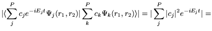
This requires the computation of the autocorrelation amplitude defined by
in time [16].
This requires the computation of the autocorrelation amplitude defined by
We found many other interesting features propagating our wave functions
in time.
First, we propagated the diagonalized eigenvectors ![]() , constructing the
functions
, constructing the
functions
![]() . We found that the autocorrelation amplitudes
. We found that the autocorrelation amplitudes
![]() for these functions are unity, even for a very long time.
This is a good test for the numerical accuracy of the propagation method.
We checked that the real and imaginary part of the autocorrelation
function oscillate with a period corresponding to
for these functions are unity, even for a very long time.
This is a good test for the numerical accuracy of the propagation method.
We checked that the real and imaginary part of the autocorrelation
function oscillate with a period corresponding to
![]() ,
where
,
where ![]() is the energy of the level
is the energy of the level ![]() .
We also tested the overlap of the propagated relaxed wave function
.
We also tested the overlap of the propagated relaxed wave function
![]() with the diagonal eigenvectors
with the diagonal eigenvectors ![]() .
These overlapping values also remained constant for a very long time,
even after the wave function bounces back many times against
the boundaries.
Projection of the propagated relaxed wave function
.
These overlapping values also remained constant for a very long time,
even after the wave function bounces back many times against
the boundaries.
Projection of the propagated relaxed wave function
![]() with product functions
with product functions ![]() , on the other hand, does depend on time.
After an initial predominance of low energies, the overlap profile shows
a steep peak centered at
, on the other hand, does depend on time.
After an initial predominance of low energies, the overlap profile shows
a steep peak centered at ![]() close to 1.6 a.u. (as is expected).
close to 1.6 a.u. (as is expected).
One can notice the presence of wiggles in the autocorrelation amplitude
at the initial steps of the time evolution
(see
Fig. 7.).
In order to understand the origin of these wiggles, we repeated
the calculations with a smaller number of mesh points, in this case
75 points separated by ![]() a.u., and the results are
plotted in
Fig. 8.
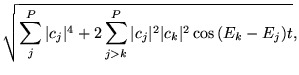
Since the eigenfunctions
a.u., and the results are
plotted in
Fig. 8.
Since the eigenfunctions ![]() obtained from the diagonalization process
constitute a complete group, we can expand the relaxed
obtained from the diagonalization process
constitute a complete group, we can expand the relaxed ![]() wave function as
wave function as
where ![]() is the dimension of the space defined in
Eq. (4).
is the dimension of the space defined in
Eq. (4).
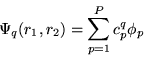
We calculated the final expression in
Eq. (26),
cutting off the number P of terms in the sum to a different
number of terms p; these results are shown in
Fig. 8.
We found that the ![]() coefficients in the
expansion (26)
have a very sharply peaked distribution around the
coefficients in the
expansion (26)
have a very sharply peaked distribution around the ![]() states
located close to the
states
located close to the ![]() function.
However, a large number of terms in the expansion
(27) are needed in order to reproduce an
exponential behavior similar to the autocorrelation amplitude of
the propagated wave function.
The relatively large size of the box allows us to study the propagation of
the wave function until long times (about 150 a.u.).
At times beyond 150 a.u., an important part of the propagating wave function
reaches the boundaries, bouncing back to the origin.
Therefore, at long times the autocorrelation amplitude is no longer
a decreasing exponential; it has an oscillatory behavior-
it shows interferences between the propagating and bouncing back
portion of the wave and other irregularities.
Surprisingly, the expansion (27) reproduces
perfectly the autocorrelation amplitude of the propagated wave function
including the oscillations and the irregularities at long times.
It is also interesting to notice how the frequency of the oscillations
is related to the size of the box.
For bigger boxes the propagating wave function takes more time to reach
the boundaries, so the frequency of the oscillations is smaller.
On the other hand, for bigger boxes the eigenvalue spectra are more dense.
Therefore, the energy differences
function.
However, a large number of terms in the expansion
(27) are needed in order to reproduce an
exponential behavior similar to the autocorrelation amplitude of
the propagated wave function.
The relatively large size of the box allows us to study the propagation of
the wave function until long times (about 150 a.u.).
At times beyond 150 a.u., an important part of the propagating wave function
reaches the boundaries, bouncing back to the origin.
Therefore, at long times the autocorrelation amplitude is no longer
a decreasing exponential; it has an oscillatory behavior-
it shows interferences between the propagating and bouncing back
portion of the wave and other irregularities.
Surprisingly, the expansion (27) reproduces
perfectly the autocorrelation amplitude of the propagated wave function
including the oscillations and the irregularities at long times.
It is also interesting to notice how the frequency of the oscillations
is related to the size of the box.
For bigger boxes the propagating wave function takes more time to reach
the boundaries, so the frequency of the oscillations is smaller.
On the other hand, for bigger boxes the eigenvalue spectra are more dense.
Therefore, the energy differences ![]() in the leading terms of
the sum (27) are smaller, tracking exactly
the oscillations in the autocorrelation amplitude.
in the leading terms of
the sum (27) are smaller, tracking exactly
the oscillations in the autocorrelation amplitude.
As we pointed out above, our result may improve by using a
finer radial mesh.
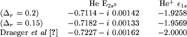
For a summary of our findings,
Table III shows our
results for the calculated energies
E
![]() for the
for the ![]() level
in He, and
level
in He, and ![]() , the energy of the
, the energy of the ![]() level in He
level in He![]() ,
for different numerical grids.
,
for different numerical grids.
|
We have developed an exact numerical method for calculating the
full spectrum of the helium atom in a box. It consists of
a direct diagonalization of the Hamiltonian in a numerical grid.
Since we have a particular interest in the doubly excited autoionizing
levels, we developed an additional method, consisting of a constrained
relaxation of the wave function.
Calculations were performed for the S-wave model He, in which
only spherical states are taken into account.
Even though our goal is not to present the best wave functions but to obtain
a good insight into the physical correlations, both methods show very good
agreement among them and with other existing calculations.
A Feshbach projection of the ![]() eigenvector is absolutely
consistent with the relaxed
eigenvector is absolutely
consistent with the relaxed ![]() wave function, proving the
reliability of the numerical procedure.
Time propagation of the relaxed wave function allows the calculation
of the autoionization rate by monitoring the autocorrelation amplitude
in time.
Furthermore, computer animations were produced to visualize the
dynamics of the autoionization process.
Work is in progress to present better numerical results, including
total close-coupling results, and for the calculations of other
processes involving transitions among the different continuum states.
wave function, proving the
reliability of the numerical procedure.
Time propagation of the relaxed wave function allows the calculation
of the autoionization rate by monitoring the autocorrelation amplitude
in time.
Furthermore, computer animations were produced to visualize the
dynamics of the autoionization process.
Work is in progress to present better numerical results, including
total close-coupling results, and for the calculations of other
processes involving transitions among the different continuum states.
Figure 1.
Figure 2.
Figure 3.
Figure 4.
Figure 5.
Figure 6.
Figure 7.
Figure 8.
![\begin{displaymath}
{\hat H} =
\left(
\begin{tabular}{ccccc}
$\left[ \,
\begi...
...
\end{tabular}\right] $\par\\
\par\end{tabular}
\right) \,
\end{displaymath}](img28.png)