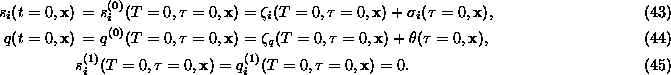
Thus, the values ![]() and
and ![]() correspond to the fixed point that the dynamical system (10)-(11)
approaches for a particular initial condition
correspond to the fixed point that the dynamical system (10)-(11)
approaches for a particular initial condition ![]() ,
, ![]() . Given the relations (7), the system
(10)-(11)
has many constants of motion. Namely, it has a total of N. Due to
(7) there are N-1 quantities
of the form:
. Given the relations (7), the system
(10)-(11)
has many constants of motion. Namely, it has a total of N. Due to
(7) there are N-1 quantities
of the form:
that are constants of motion for the system (10)-(11). On the other hand, the total mass
where ![]() and
and ![]() are the masses of species
are the masses of species ![]() and Q, respectively, is also a constant for the system (10)-(11)
(this is a consequence of our assumption that all feeding terms occur on
the slow timescale). Therefore, the N+1-dimensional dynamical system
(10)-(11)
has N constants of motion. Each level set (i.e., the set
of points in the space of concentrations for which each of the N
constants has a particular given value) is a one-dimensional curve that
generically intersects the N-dimensional set of fixed points (20)
at isolated points. Notice that, since all the constants are linear in
the concentrations, the level sets are straight lines. Given an initial
condition that belongs to one particular level set, then the system evolves
according to Eqs. (10)-(11)
without ever leaving that level set. Since the level sets are one-dimensional
objects (straight lines in this case), the only attractors they can contain
are fixed points. Assuming that each level set intersects the set of fixed
points (20) only once (which is consistent
with our assumption that all the points on the set of fixed points are
attracting), then the fixed point that each initial condition approaches
is uniquely determined: it is the one defined by the same values for the
constants of motion as the initial condition. We schematically depict this
situation in Fig. 2 (a).
and Q, respectively, is also a constant for the system (10)-(11)
(this is a consequence of our assumption that all feeding terms occur on
the slow timescale). Therefore, the N+1-dimensional dynamical system
(10)-(11)
has N constants of motion. Each level set (i.e., the set
of points in the space of concentrations for which each of the N
constants has a particular given value) is a one-dimensional curve that
generically intersects the N-dimensional set of fixed points (20)
at isolated points. Notice that, since all the constants are linear in
the concentrations, the level sets are straight lines. Given an initial
condition that belongs to one particular level set, then the system evolves
according to Eqs. (10)-(11)
without ever leaving that level set. Since the level sets are one-dimensional
objects (straight lines in this case), the only attractors they can contain
are fixed points. Assuming that each level set intersects the set of fixed
points (20) only once (which is consistent
with our assumption that all the points on the set of fixed points are
attracting), then the fixed point that each initial condition approaches
is uniquely determined: it is the one defined by the same values for the
constants of motion as the initial condition. We schematically depict this
situation in Fig. 2 (a).
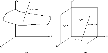
Figure: Integration of the fast equations. The straight line
is the level set which is uniquely determined by the values of the (in
this case two) constants of motion. The arrow indicates how the system
evolves in time. Each level set intersects the manifolds depicted in Fig.
1 at isolated points. The first point
of intersection provides the initial condition for the reduced (slow) evolution
equations. (a) The case of one fast reversible reaction. (b) The case of
one fast irreversible reaction.
The system with k'=0 has the same N constants of motion
as before. But now, each level set may intersect the set of fixed points
more than once. This is shown schematically for the case with three species
in Fig 2 (b). In this case, the set of
fixed points are the three planes defined by ![]() ,
, ![]() and q=0. A generic straight line in the three-dimensional space
and q=0. A generic straight line in the three-dimensional space ![]() will intersect all three planes. Therefore, not all the fixed points can
be regarded as stable. Of course, the only fixed points (and initial conditions)
that are physically relevant are those for which
will intersect all three planes. Therefore, not all the fixed points can
be regarded as stable. Of course, the only fixed points (and initial conditions)
that are physically relevant are those for which ![]() , and each level set can contain at most two such fixed points. This is
due to the fact that the level sets are straight lines (see Fig.fig:integ
(b)). The continuity of the flow guarantees then that one of these two
fixed points is stable. Thus, given an initial condition, also in this
case there is a unique fixed point of the dynamical system (10)-(11)
that the system approaches eventually in time. This fixed point is the
initial condition for the reduced set of equations.
, and each level set can contain at most two such fixed points. This is
due to the fact that the level sets are straight lines (see Fig.fig:integ
(b)). The continuity of the flow guarantees then that one of these two
fixed points is stable. Thus, given an initial condition, also in this
case there is a unique fixed point of the dynamical system (10)-(11)
that the system approaches eventually in time. This fixed point is the
initial condition for the reduced set of equations.
As mentioned in the paper, the reduction may also be obtained directly
by looking for an algebraic relationship among the variables (see Sec.
V of the paper). When this is done, the information on which is the initial
condition for the ``slow'' (reduced) equations is lost. However, it is
still possible to integrate the fast portion of all the equations simultaneously
as done in this Secion. Given that it is assumed that diffusion acts on
the slow timescale, this means solving a set of ODE's. The problem when
doing this is that the algebraic relationship that is kept in general may
not coincide with the manifold of fixed points for the fast equations.
Thus, once the fast ODE's are integrated, it is necessary to look for the
point on the ``slow'' manifold defined by the algebraic relationship ![]() that is closer to the fixed point that the real initial condition approaches
under the fast dynamics. This point may then be used as the initial condition
for the reduced (slow) equations.
that is closer to the fixed point that the real initial condition approaches
under the fast dynamics. This point may then be used as the initial condition
for the reduced (slow) equations.