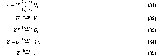
and later in ,
where a variety of patterns was observed. We will consider the four variable
model presented in ,
which is given by the following set of reactions
and later in ,
where a variety of patterns was observed. We will consider the four variable
model presented in ,
which is given by the following set of reactions
where ![]() ,
, ![]() ,
, ![]() and
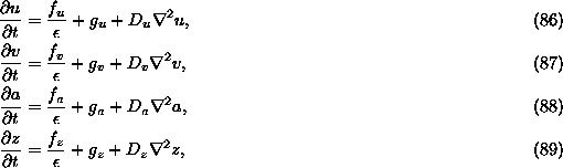
and ![]() . Including diffusion, we get from this model the following dynamical equations:
. Including diffusion, we get from this model the following dynamical equations:
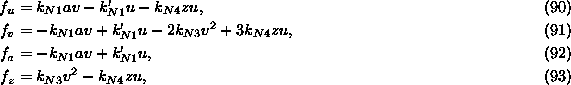
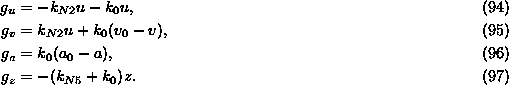
where
and
In writing Eqs. (94)-(97)
we are assuming that the species V and A are fed into the
system and this happens at the same rate at which all of the species are
removed ( ![]() ).
).
In this Section we apply the methods of Sec. V of the paper to Eqs.
(86)-(89)
to obtain the equations describing the slow time dynamics for this model.
In order to make this calculation more specific, we consider the parameter
values that are used in the experiments when replicating spot pattern is
observed: ![]() ,
, ![]() ,
, ![]() ,
, ![]() ,
, ![]() ,
, ![]() . It is not completely clear what the values of
. It is not completely clear what the values of ![]() and
and ![]() actually are inside the gel where the reaction takes place. We will consider
actually are inside the gel where the reaction takes place. We will consider ![]() and
and ![]() . Inspired by the reduction of the ODE's performed by Gáspár
and Showalter, we seek a reduction of the PDE's (86)-(89)
in which the variables a and z are eliminated in favor of
u and v. To this end we follow the steps of Sec. V of the
paper considering
. Inspired by the reduction of the ODE's performed by Gáspár
and Showalter, we seek a reduction of the PDE's (86)-(89)
in which the variables a and z are eliminated in favor of
u and v. To this end we follow the steps of Sec. V of the
paper considering ![]() ,
, ![]() ,
, ![]() and
and ![]() . We find:
. We find:
Since the Z species is iodine, which binds to the gel, its diffusion
coefficient may be neglected. For the sake of simplicity, we will also
neglect the diffusion term of A. Inserting the expansions ![]() and
and ![]() in Eqs. (86)-(87)
we find:
in Eqs. (86)-(87)
we find:
where we have defined ![]() ,
, ![]() ,
, ![]() ,
, ![]() ,
, ![]() ,
, ![]() and
and ![]() . Now, the whole calculation is consistent provided that
. Now, the whole calculation is consistent provided that ![]() and
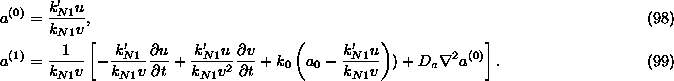
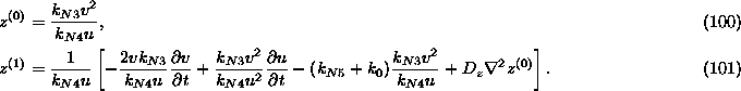
and ![]() . As we may see from Eqs. (99) and (101),
both
. As we may see from Eqs. (99) and (101),
both ![]() and
and ![]() contain terms that are proportional to
contain terms that are proportional to ![]() and
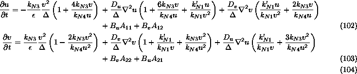
and ![]() . These time derivatives may get large given that Eqs. (102)-(103)
contain terms which are proportional to
. These time derivatives may get large given that Eqs. (102)-(103)
contain terms which are proportional to ![]() . However, the existence of more than two timescales is of help in this
case. Assuming that the right-hand-side of Eqs. (99),
(101), (102)
and (103) are dominated by the terms
proportional to
. However, the existence of more than two timescales is of help in this
case. Assuming that the right-hand-side of Eqs. (99),
(101), (102)
and (103) are dominated by the terms
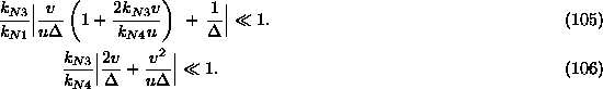
proportional to ![]() , we may rewrite the conditions
, we may rewrite the conditions ![]() and
and ![]() as:
as:
For the parameter values we are considering it is ![]() and
and ![]() . Thus, provided that v/u does not become too large, the
conditions (105) and (106)
are satisfied and the calculation is self-consistent.
. Thus, provided that v/u does not become too large, the
conditions (105) and (106)
are satisfied and the calculation is self-consistent.